Positive Gradients, Negative Gradients

+ the Importance of Pre-Training Priors

In Reinforcement Learning (RL), particularly when fine-tuning Large Language Models (LLMs), we often treat positive and negative feedback as two sides of the same coin. Mathematically, the transition from positive to negative examples in the loss function is smooth. Whether you are maximizing the log-probability of a “good” response or minimizing the log-probability of a “bad” one, the gradient updates look qualitatively similar. However, their effects on the model couldn’t be more different.

Understanding this asymmetry explains why RL often leads to model collapse and why the prior established during pre-training deserves much more attention than it currently gets. The core difference lies in how the gradients affect the output distribution.

When we train on on-policy positive examples, we are reinforcing samples that already lie in high-density regions of the output distribution (since the model generated them). Applying a positive gradient here effectively says, “Do exactly this, but more.” This creates a “rich get richer“ effect. The model pushes the peaks of the probability distribution even higher. Because probability must sum to 1, this mass is taken from the tail of the distribution. The result is a rapid reduction in entropy and a collapse in diversity. The model becomes extremely confident in its current path.

Negative gradients operate differently. When we apply a negative gradient to an on-policy sample (which, again, is likely a high-probability error), we are chopping off the peak. The optimization process is forced to redistribute that probability mass elsewhere to maintain normalization. The loss function doesn’t specify where that mass should go, only that it cannot stay at the erroneous location. This forces the model to lift the lower-probability regions, naturally flattening the distribution and increasing the entropy. It’s important to note here that when the probability gets redistributed, it still generally remains within the support of the output distribution, with lower-prior regions receiving less of the redistribution.

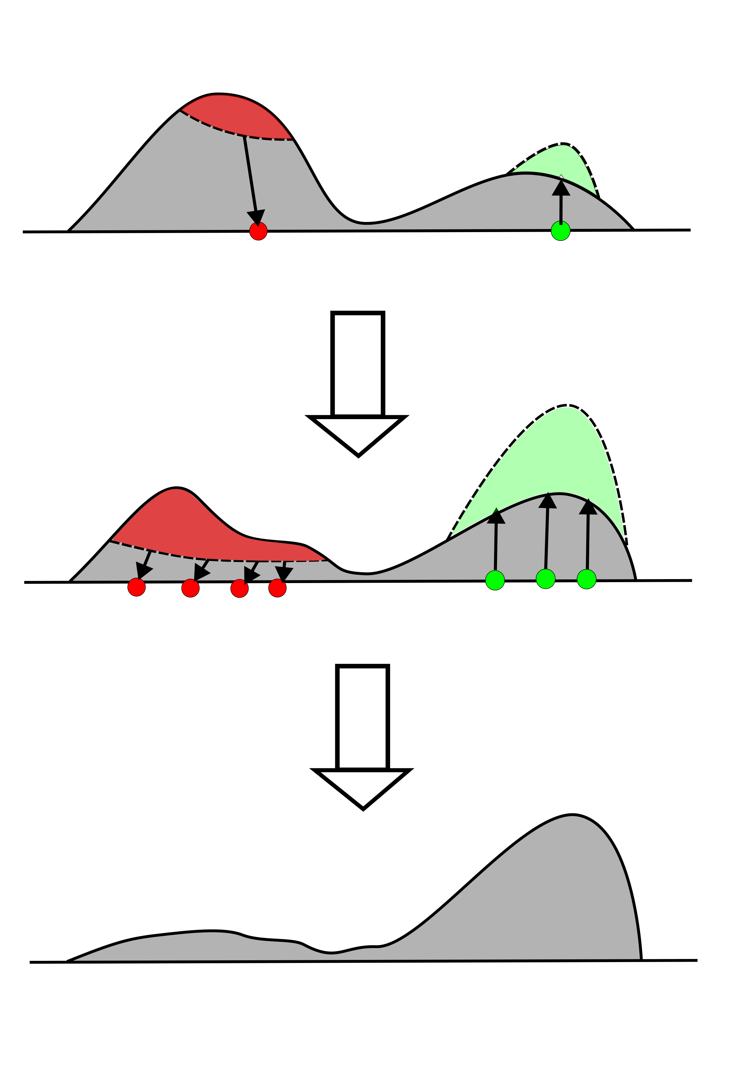
The figure below illustrates the effects of positive (green) and negative (red) on-policy examples. The positive examples locally “absorb” the probability density, while the negative examples “expel” the density.

The effect of positive and negative examples on the probability density

Evidence from the Literature

The paper “The Surprising Effectiveness of Negative Reinforcement in LLM Reasoning” investigates this exact phenomenon. The authors find that positive on-policy examples quickly collapse entropy. While this might sharpen the model’s best guess (improving pass@1), it destroys the diversity needed for test-time compute scaling (hurting pass@k for large k).

Conversely, negative examples effectively prune the “wrong” modes without collapsing the distribution. They maintain higher entropy, preserving the model’s ability to generate diverse candidate solutions, which is critical for difficult reasoning problems where the first guess isn’t always right.

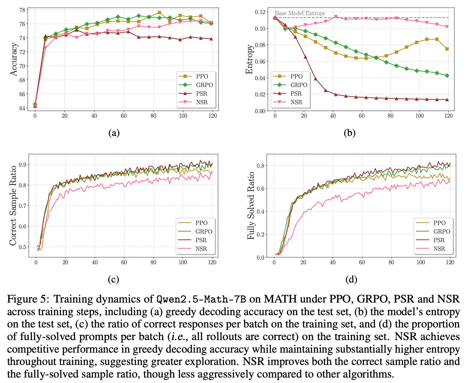
Figure 5 below shows that Positive Sample Reinforcement (PSR, on-policy RL on positive examples only) collapses the entropy and leads only to a small increase in accuracy, while Negative Sample Reinforcement (NSR, on-policy RL on negative examples only) avoids the entropy collapse and reaches the accuracy levels similar to PPO/GRPO. The authors make an analogy PSR being Exploitation and NSR being Exploration. PSR reinforces discovered positive behaviors, while NSR shifts the probability away from discovered negative behaviors and the allocation of this probability to other outputs causes some exploration. An important caveat is that NSR redistributes probability within the support of the policy, so the extent of exploration is fairly limited.

Figure 5 from The Surprising Effectiveness of Negative Reinforcement in LLM Reasoning

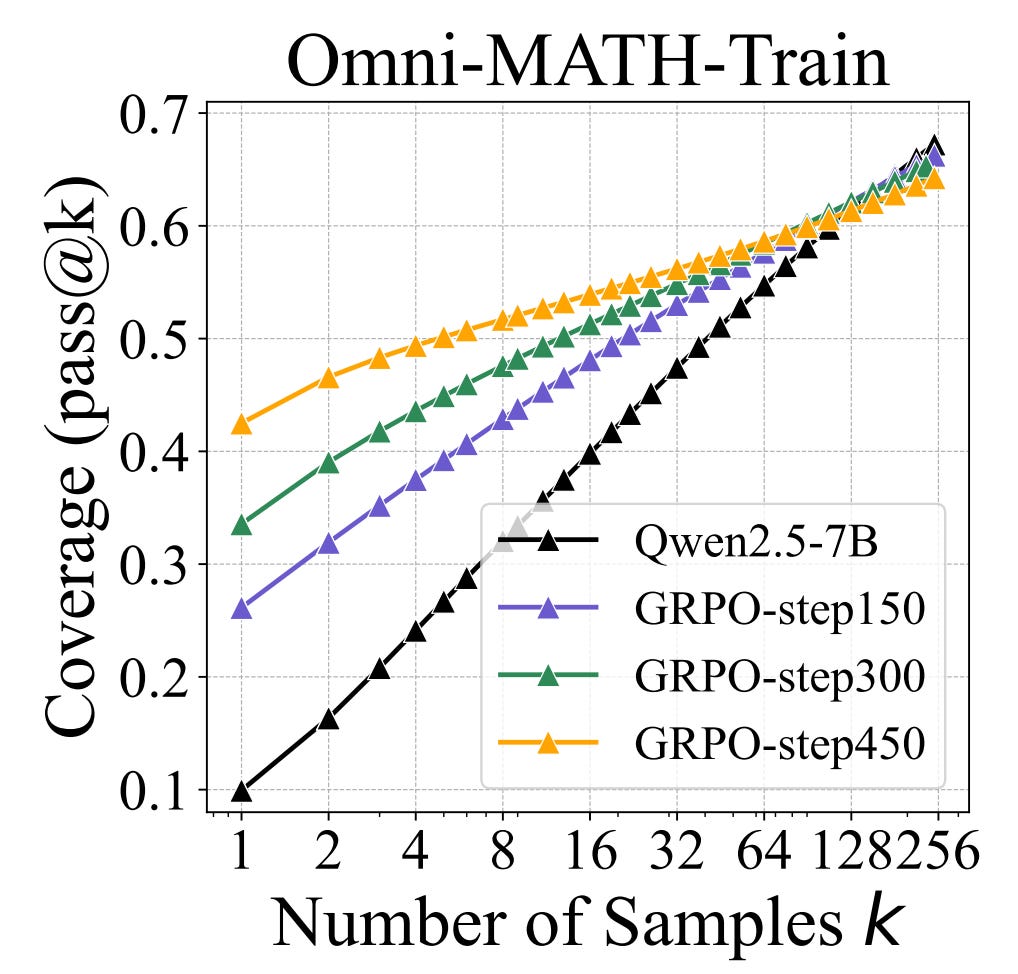
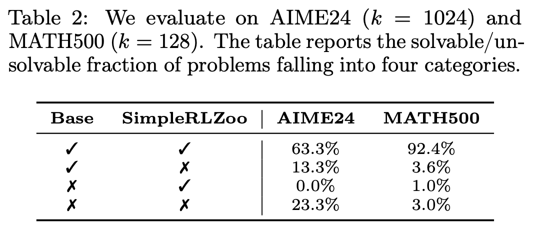
This aligns with findings from “Does Reinforcement Learning Really Incentivize Reasoning Capacity in LLMs Beyond the Base Model?”. This paper suggests that RL doesn’t teach the model new reasoning behaviors. Instead, it prioritizes useful patterns that already exist after pre-training (via positive gradients) and prunes incorrect ones (via negative gradients). Figure 1 illustrate this - RLVR training increases pass@1 rates, but reduces pass@k rates for large k>64. Additionally, Table 2 shows that for AIME24 there isn’t a single problem which the base model couldn’t solve (with a large number of samples k=1024), but the post-RLVR model can solve. Similarly, for MATH500 the post-RLVR model gains the ability to solve only 1% of problems which couldn’t be solved by the base model, but at the same time it loses the ability to solve 3.6% of problems which the pre-trained model could solve.

Figure 1 from “Does Reinforcement Learning Really Incentivize Reasoning Capacity in LLMs Beyond the Base Model?”

Table 2 from “Does Reinforcement Learning Really Incentivize Reasoning Capacity in LLMs Beyond the Base Model?”

The bottom line is fairly clear - on-policy RVLR reliably increases the accuracy (pass@1), but it reduces generation diversity, leading to a reduction in pass@k for large k. This training recipe can give us a reliable solver of simple problems, but it won’t produce a model which can get even close to pushing the frontier of knowledge.

Training Example Sources: On-Policy vs Off-Policy

The patterns described above apply only to on-policy training data. Off-policy training examples are substantially different.

Off-policy positive examples are used for Supervised Fine-Tuning (SFT) and are generally known to improve both accuracy and diversity (unless we overfit by training for too many epochs). If we show the model a “Gold” solution that it currently assigns low probability to, we are forcing it to expand the support of its distribution. This increases diversity by teaching the model a new mode it hadn’t discovered on its own. The main downside of off-policy positive examples is that they by themselves don’t induce good generalization due to lack of pruning via negative on-policy examples.

Off-policy negative examples are not well understood. My intuition here is that if you penalize a behavior which the model essentially never does (low probability mass), the gradient should be negligible. But such examples are a core part of some successful DPO-baed training recipes and their effect deserves a more thorough investigation.

We end up with the following priority list of types of training examples:

1. Negative On-Policy: High utility. Prunes errors, maintains diversity.

2. Positive Off-Policy: High utility. Expands diversity, teaches new behaviors.

3. Positive On-Policy: Mixed utility. Sharpens pass@1 but risks mode collapse.

4. Negative Off-Policy: Unclear utility. Needs more research.

The Prior

If on-policy RL is primarily a mechanism for reinforcing existing good behaviors (sharpening peaks) or pruning wrong ones (cutting peaks), then we are left with an uncomfortable conclusion: it can’t learn qualitatively new behaviors.

The irony here is that a tight prior from pre-training is the very thing that makes RL possible for LLMs in the first place. After pre-training most of the output probability gets concentrated in just a few tokens and this effectively shrinks the action space to 2-5 options at each position, compared to the full unconstrained vocabulary size of ~130k tokens. It would be hopeless to start RL training from a uniform prior over a discrete action space with 130k elements, especially when you consider long trajectories with only terminal rewards.

The effectiveness of RL post-training pipeline is strictly bounded by the support of the prior produced by pre-training. To break these bounds, we cannot simply rely on standard LLM RL with high-temperature sampling. We have two main paths forward:

1. Fix the prior: We can encourage significantly more diversity during pre-training, ensuring the initial distribution extensively covers the space of responses. Synthetic data augmentation for pre-training could potentially help here, but we’d need to be careful to avoid regurgitating the data without substantially transforming it. Also, this introduces a risk of capability dilution if the output distribution includes too many low-quality outputs.

2. Break out from the prior: A much more promising path, in my opinion. We need advanced exploration methods that go beyond the model’s current policy (true off-policy exploration) to expand the support of the output distribution, rather than just reshaping what is already there. The most useful thing would be to generate positive examples which are slightly off-policy to gradually expand the output distribution towards correct responses.