Bandits vs Reinforcement Learning from Human Feedback

Reinforcement Learning from Human Feedback (RLHF) has caused a surge of interest in Reinforcement Learning (RL) algorithms, specifically the Proximal Policy Optimization (PPO) [1], popularized for RLHF by the InstructGPT [2] paper. The success of InstructGPT and its commercial successor ChatGPT has made PPO the de facto standard algorithm for LLM fine-tuning. But a recent paper [3] questioned whether the complexity of PPO is necessary, and has shown that a simpler REINFORCE algorithm applied to a contextual bandit model works better. In this post, I’ll share the main ideas from this paper and discuss the differences between using contextual bandit and multi-step RL for LLM fine-tuning.

REINFORCE paper

Cohere has recently published a paper “Back to Basics: Revisiting REINFORCE Style Optimization for Learning from Human Feedback in LLMs” [3], in which they argue that REINFORCE should replace PPO as the default RLHF algorithm. Moreover, they suggest that multi-step RL algorithms aren’t necessary for LLM fine-tuning and simpler single-step contextual bandit algorithms can be used instead. Even though REINFORCE is usually used as a multi-step RL algorithm, this paper uses its simplified contextual bandit version. Their arguments center around the fact that PPO was developed for different types of problems like robotics and control, which have their own challenges distinct from RLHF. Quoting from the paper:

We note that PPO, as an approach, emphasizes stability across iterations, aiming to train an effective policy with the premise of small, stable updates. PPO was designed for a regime where off-policy gradient updates are large enough to introduce instability. This regime dominates traditional Deep-RL benchmarks [...] However, in this work, we posit that the setting of RLHF, which involves fine-tuning a pre-trained LLM, is lacking in these characteristics.

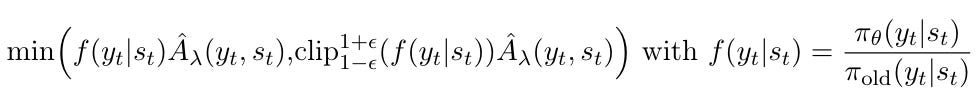
They identify 3 distinct components of PPO (see the PPO objective above) and show evidence that each of these components is unnecessary for RLHF of pre-trained LLMs. The 3 components are:

1. Clipped off-policy probability ratios. They found that clipping was applied <5% of the time in their RLHF runs, so it’s rarely necessary. They found the algorithm to work better when clipping was turned off. This shows that large off-policy updates are uncommon when fine-tuning pre-trained LLMs.

   1. Moreover, they found that the probability ratios were close to 1 most of the time, so they removed the ratios from the loss without any impact on learning stability or quality. This switched the algorithm from being off-policy to a simpler on-policy PG algorithm.

2. Generalized Advantage Estimation (GAE) [4] and separate value function. The advantage term in PPO is estimated by GAE, which bootstraps from the learned value function to reduce variance. GAE has a hyperparameter lambda, which controls the bias-variance tradeoff. Turns out that setting lambda=1 results in the best performance. Under this setting the algorithm completely ignores the value function and just uses the reward model (highest variance, lowest bias).

3. Multi-step RL modeling. In PPO it’s assumed that text generation is a token-by-token multi-step process. The paper shows that this is unnecessary and a simpler bandit approach that models the whole response as a single step consistently outperforms the multi-step RL approach. This allows us to avoid dealing with partial responses and only consider full responses.

One of the core arguments about the ineffectiveness of PPO for LLM fine-tuning is related to its focus on reducing variance. It turns out that the RLHF of LLMs is much less exposed to high variance of gradients than classical deep RL environments, so it’s not worth it to increase bias for the sake of reducing variance. The main reasons for the low gradient variance during RLHF for pre-trained LLMs are:

1. High quality of pre-trained LLMs. Most classical RL environments cannot pre-train the agents before starting RL training, so the initial policy is very poor and requires variance reductions to prevent destructively large gradient updates.

2. Small size of effective action space. While the full action space size at each decoding step is equal to the number of tokens in the dictionary (on the order of 10k-100k), pre-training leads to a strong concentration of probability mass in just a handful of tokens, making the action space effectively smaller. In their experiments, 60% of probability mass was concentrated in the top token and 90%+ in the top 16 tokens.

Comparison of RL and Bandits for LLM

Why do we even have a choice of whether to use RL or bandit models for LLMs? After all, nobody in their right mind would consider modeling a robot or a chess agent as a bandit environment. It’s because in LLMs the transition dynamics are very simple and deterministic. The state is modeled as the sequence of previous tokens and the action is the choice of the next token to decode. This leads to a simple state transition rule: append the action token to the list of previous tokens. Since no new information is revealed after each token, selecting the tokens one by one is equivalent to pre-committing to a sequence of tokens and executing them one by one. This does not prevent us from updating the token probabilities autoregressively by feeding each new token back into the model before generating the next token.

The simplest definition of a contextual bandit environment is a single-step Markov Decision Process (MDP). The agent observes the state (context), executes an action, and receives a reward. Then, the episode terminates and the next episode arrives. A crucial assumption in contextual bandits is that each episode is independent of the actions taken during other episodes. RL, on the other hand, deals with multi-step MDPs in which several state-action-reward steps are repeated until the episode terminates. The state transitions are allowed to depend on the actions.

To better understand the structural differences between RL and bandit approaches, let’s examine their Policy Gradient  (PG, [5]) objectives more closely. PPO uses an off-policy PG expression, while REINFORCE uses an on-policy PG, but this distinction is orthogonal to using RL vs bandits, so I will use on-policy PG in both RL and bandit examples. I will strip away all bells and whistles of the algorithms and consider the simplest reasonable RL and bandit formulations for LLM fine-tuning to illustrate the difference between them.

First, a simple RL objective for a single trajectory of length T looks like this:

\(\sum_{t=1}^T A(y_t|x,y_1,...,y_{t-1})\ln \pi (y_t|x,y_1,...,y_{t-1})\)

Compare this to a bandit objective:

\(A(y,x) \ln \pi (y|x) = A(y,x) \ln \prod_{t=1}^T \pi (y_t|x,y_1,...,y_{t-1})= \sum_{t=1}^T A(y,x)\ln \pi (y_t|x,y_1,...,y_{t-1})\)

The objective functions are remarkably similar. The main difference is that the multi-step RL uses a different advantage value at each step, estimated by an advantage function with partial responses as inputs, usually implemented via a learned value function. On the other hand, the bandit model uses the same advantage value for each step, and the advantage function takes full response as an input. In [3] the bandit advantage is implemented through the Reinforce Leave One Out (RLOO) algorithm, which removes the need for a learned value/baseline function. It generates multiple responses for the same prompt and uses the average reward model scores of other responses as a baseline to calculate the advantage. The core difference between RL and bandit losses is whether the advantage function takes full or partial responses as an input.

The most obvious disadvantage of the bandit approach to LLMs is that they only attribute the reward to the full response, not individual tokens. This is OK for vanilla RLHF, but it would not be efficient for more advanced approaches that attribute some reward values to individual tokens. Dense token-level feedback could be useful to reduce hallucinations and toxicity [6], or reward the model for making partial progress [7], [8].

The table below summarizes the pros and cons of using multi-step RL and bandits for LLM fine-tuning.

It’s worth mentioning that the InstructGPT paper [2] has caused a good amount of confusion in the community about whether they used a bandit or an RL setup for RLHF fine-tuning. Without open source code available, the community was left to guess how exactly RLHF was implemented in InstructGPT (and later in ChatGPT and GPT–4). This is not unlike religious scholars arguing over the meaning of passages from the Bible. My bet is on OpenAI having used multi-step RL and just not being clear in describing it.

Evidence for InstructGPT using multi-step RL:

1. The paper refers to a separate reward model and value model. This makes sense only in a multi-step RL world.

2. The paper mentions GAE, which applies only to multi-step RL

Evidence for InstructGPT using bandits:

1. Quote from the paper: “The environment is a bandit environment which presents a random customer prompt and expects a response to the prompt”.

2. John Schulman (the main author of the PPO paper and one of the core contributors to InstructGPT) said in a podcast interview shortly after the release of the InstructGPT paper: "...we've been just looking at a contextual bandit problem. ... you get a query and you output a response and then that response gets a reward. So if we had a multi-step process, such as a conversation where you can't assign a reward until the very end of the conversation ... You would probably have to ... train a Q function. I think we'll have to start exploring this at some point soon, but so far we haven't"

Framing LLM fine-tuning as a bandit problem opens the door to future applications of a rich set of bandit methods to LLMs. Contextual bandits are much simpler than RL mathematically, so a wider range of rigorous methods were developed. RL has often followed a more relaxed approach with fewer conclusive proofs and stronger reliance on empirical results. Some examples of bandit-based methods that could be applied to LLMs: offline learning [9], offline evaluation [10], and exploration [11]. Another development that I expect to happen is the customization of contextual bandit methods to work with a unique action space of LLMs: variable-size discrete action space. LLMs generate tokens until the EOS token is returned (or the maximum generation length is reached). Each token can be modeled as a discrete choice along one of the dimensions of the action space, but this leads to a variable dimensionality of the action space, depending on the number of generated tokens. The simple approach used now is to take a sequential product of individual token probabilities as the probability of the response, but more specialized approaches could be useful.

Recap

1. LLM can be framed as a multi-step MDP and solved with Reinforcement Learning methods. Or it can be framed as a single-step MDP and solved with Contextual Bandit methods.

2. PPO applied to a multi-step MDP is the de-facto standard approach to RLHF, but a recent paper showed that a simpler REINFORCE algorithm applied to a single-step contextual bandit MDP outperforms PPO.

3. More research into Contextual Bandit methods for RLHF is likely to come out in the coming years, improving both training and evaluation.

References

1. Schulman, John, Filip Wolski, Prafulla Dhariwal, Alec Radford, and Oleg Klimov. "Proximal policy optimization algorithms." arXiv preprint arXiv:1707.06347 (2017).

2. Ouyang, Long, Jeffrey Wu, Xu Jiang, Diogo Almeida, Carroll Wainwright, Pamela Mishkin, Chong Zhang et al. "Training language models to follow instructions with human feedback." Advances in neural information processing systems 35 (2022): 27730-27744.

3. Ahmadian, Arash, Chris Cremer, Matthias Gallé, Marzieh Fadaee, Julia Kreutzer, Ahmet Üstün, and Sara Hooker. "Back to Basics: Revisiting REINFORCE Style Optimization for Learning from Human Feedback in LLMs." arXiv preprint arXiv:2402.14740 (2024).

4. Schulman, John, Philipp Moritz, Sergey Levine, Michael Jordan, and Pieter Abbeel. "High-dimensional continuous control using generalized advantage estimation." arXiv preprint arXiv:1506.02438 (2015).

5. Weng, Lilian. "Policy Gradient Algorithms." lilianweng.github.io (2018)

6. Wu, Zeqiu, Yushi Hu, Weijia Shi, Nouha Dziri, Alane Suhr, Prithviraj Ammanabrolu, Noah A. Smith, Mari Ostendorf, and Hannaneh Hajishirzi. "Fine-grained human feedback gives better rewards for language model training." Advances in Neural Information Processing Systems 36 (2024).

7. Paul, Debjit, Mete Ismayilzada, Maxime Peyrard, Beatriz Borges, Antoine Bosselut, Robert West, and Boi Faltings. "Refiner: Reasoning feedback on intermediate representations." arXiv preprint arXiv:2304.01904 (2023).

8. Lightman, Hunter, Vineet Kosaraju, Yura Burda, Harri Edwards, Bowen Baker, Teddy Lee, Jan Leike, John Schulman, Ilya Sutskever, and Karl Cobbe. "Let's Verify Step by Step." arXiv preprint arXiv:2305.20050 (2023).

9. Joachims, Thorsten, Adith Swaminathan, and Maarten De Rijke. "Deep learning with logged bandit feedback." In International Conference on Learning Representations. 2018.

10. Dudík, Miroslav, Dumitru Erhan, John Langford, and Lihong Li. "Doubly robust policy evaluation and optimization." (2014): 485-511.

11. Hao, Botao, Tor Lattimore, and Csaba Szepesvari. "Adaptive exploration in linear contextual bandit." In International Conference on Artificial Intelligence and Statistics, pp. 3536-3545. PMLR, 2020.